The loss function determines the output of the neural network. The output layer is not necessarily trained to be equal to the target.

Let’ define $z$ as the output of the last linear layer (no activation):

$z = [z_1, \dots, z_h, \dots, z_H]$

Before the loss can be calculated some non-linear transformations may be needed. For example, a classification problem requires the output to be interpreted as a probability for the class assigned to the output node. Therefore the output is skewed to fit in the range [0, 1].

It should be noted that this need is not limited to the classification tasks. In a regression problem for predicting values with high dynamic ranges, the same error does not have the same effect for all predictions, e.g. prediction error of \$1 for a product of \$1000 is small and acceptable, but the same error when the product is \$2 is not good. The simplest solution in such situation is to use logarithm, but this is out of the scope of this tutorial.

The standard loss functions are crossentropy (for classification) and mean squared error (for regression). The non-linearity could be added as a separate layer or could be part of the Loss calculation. This changes the actual output and loss.

Sigmoid and softmax non-linearities

The output $z$ can be converted to probability like values $\hat{y}$ in two ways:

through sigmoid, $\hat{y}_h = p(c_h) = \mathrm{sigmoid}(z) = \frac{1}{1 + \exp(-z_h)} = \frac{\exp(z_h)}{\exp(z_h)+\exp(0)}$ - different outputs are independent, used for binnary classifier, could be used for multilabel-multiclass categorisation. Each output node represents the probability of a separate binnary variable (label).
through softmax, $\hat{y}_h = p(c_h) = \mathrm{softmax}(z) = \frac{\exp(z_h)}{\sum{\exp(z_j)}}$ - all outputs sum to one, used for multiclass categorisation. All output node values represent a probability distribution of single variable (class, category)

where

$c_h$ is the category assigned to the $h$-th output node
$\hat{y_h}$ is the estimated likelihood of $c_h$

import torch
from torch import tensor

# Available categories
c = ['male', 'female']

# Generate test data - example output z of the last linear layer
# Two output features (H=2)
z = tensor([0., 5.])
z, z.shape

(tensor([0., 5.]), torch.Size([2]))

def sigmoid(x):
    return 1. / (1 + torch.exp(-x))

def softmax(x):
    # print('Input shape:', x.shape, 'Sum shape:', torch.exp(x).sum(dim=-1, keepdim=True).shape )
    return torch.exp(x) / torch.exp(x).sum(dim=-1, keepdim=True)

sigmoid(z), softmax(z)

(tensor([0.5000, 0.9933]), tensor([0.0067, 0.9933]))

from fastcore.test import test_close

test_close(softmax(z), torch.softmax(z, dim=-1))

test_close(sigmoid(z), torch.sigmoid(z))

Neural networks are designed to process data in batches. This means that the input (and the output) will have one additional dimension for the samples.

# Generate test data - batch outputs of the last linear layer
# Six items (N=6) and two output features (H=2)
zz = tensor([[1, 10],
             [2, -2],
             [2, 2],
             [0, 2],
             [4.5, 5],
             [0, 0]
            ])
zz, zz.shape

(tensor([[ 1.0000, 10.0000],
         [ 2.0000, -2.0000],
         [ 2.0000,  2.0000],
         [ 0.0000,  2.0000],
         [ 4.5000,  5.0000],
         [ 0.0000,  0.0000]]),
 torch.Size([6, 2]))

softmax(zz)

tensor([[1.2339e-04, 9.9988e-01],
        [9.8201e-01, 1.7986e-02],
        [5.0000e-01, 5.0000e-01],
        [1.1920e-01, 8.8080e-01],
        [3.7754e-01, 6.2246e-01],
        [5.0000e-01, 5.0000e-01]])

test_close(sigmoid(zz), torch.sigmoid(zz))

test_close(softmax(zz), torch.softmax(zz, dim=-1))

Targets

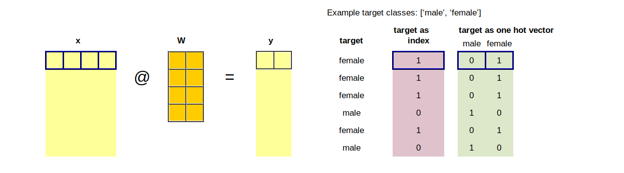
The true classes/labels are needed in addition to the model predictions in order to calculate the loss. A target could be provided as a number - the index of the true class, or as a vector - one hot encoding.

# Generate test targets
# y = torch.randint(0, 2, (6,))
y = tensor([1, 1, 1, 0, 1, 0])
yy = torch.zeros((6,2))
yy[range(len(yy)), y] = 1
print('Target as index: ', y)
print('The same, one hot encoding:\n', yy)

Target as index:  tensor([1, 1, 1, 0, 1, 0])
The same, one hot encoding:
 tensor([[0., 1.],
        [0., 1.],
        [0., 1.],
        [1., 0.],
        [0., 1.],
        [1., 0.]])

Crossentropy loss

Let’s denote:

$y_{ih}$ is 1 if for sample $i$ the true class is $c_h$ and 0 otherwise (one hot encoding).
$y_i = \mathrm{argmax}(y_{ih})$ is the index of the true class for sample $i$ from the batch.
$\hat{y}_{ih}$ is the estimated likelihood of $c_h$ for sample $i$
$\hat{y}_{i} = \hat{y}[i, j=\mathrm{argmax}(y_{ih})]$ is the estimated likelihood of the true class for sample $i$

Crossentropy loss can be defined for binnary cases as follows:

$\mathbb{L} = - \sum_{i=1}^N{[ y_i \ln(\hat{y_i}) + (1 -y_i) \ln(1 -\hat{y}_i)]}$

$\mathbb{L} = - \sum_{i=1}^N{[ y_i \ln(p(c_i)) + (1 -y_i) \ln(1 -p(c_i))]}$

$\mathbb{L} = - \sum_{i=1}^N{[ y_i \ln(\mathrm{sigmoid(z_i)}) + (1 -y_i) \ln(1 -\mathrm{sigmoid(z_i)})]}$

Crossentropy loss can be defined for multiclass cases as follows:

$\mathbb{L} = - \sum_{i=1}^N \sum_{h=1}^H{y_{ij}\ln(\hat{y}_{ih}) }$

$\mathbb{L} = - \sum_{i=1}^N \sum_{h=1}^H{y_{ij} \ln(p(c_{ih})) }$

$\mathbb{L} = - \sum_{i=1}^N \sum_{h=1}^H{y_{ij} \ln(\mathrm{softmax(z_{ih})}) }$

$\mathbb{L} = - \sum_{i=1}^N {\ln(\hat{y}_{i}) } = - \sum_{i=1}^N { \ln(p(c_{i})) } = - \sum_{i=1}^N { \ln(\mathrm{softmax(z_{i})}) }$

We can notice that:

Only the softmax of the true classes is needes as the other outputs are multiplied by zero ($y_{ij}=0$ for one hot encoded class different than $y_i$)
We need logarithm of the softmax, so the expression contain $\log(\exp())$ and can be simplified

Log(Softmax) calculation

def log_softmax(x):
    '''Logarithm of predicted probabilities calculated from the output'''
    return softmax(x).log()

test_close(log_softmax(z), torch.log_softmax(z, dim=-1))

test_close(log_softmax(zz), torch.log_softmax(zz, dim=-1))

def log_softmax2(x):
    return x - x.exp().sum(dim=-1, keepdim=True).log()

test_close(log_softmax2(z), torch.log_softmax(z, dim=-1))

test_close(log_softmax2(zz), torch.log_softmax(zz, dim=-1))

def logsumexp(x):
    # a = x.max(dim=-1, keepdim=True)[0]
    # return a + (x-a).exp().sum(dim=-1, keepdim=True).log()
    a = x.max(dim=-1)[0]
    return a + (x-a[...,None]).exp().sum(dim=-1).log()

test_close(logsumexp(z), torch.logsumexp(z, dim=-1))

test_close(logsumexp(zz), torch.logsumexp(zz, dim=-1))

def log_softmax3(x):
    return x - logsumexp(x).unsqueeze(-1)

test_close(log_softmax3(z), torch.log_softmax(z, dim=-1))

test_close(log_softmax3(zz), torch.log_softmax(zz, dim=-1))

Cross-entropy loss for log-probabilities, `F.nll_loss()`

$\mathbb{L} = - \sum_{i=1}^N \sum_{h=1}^H{y_{ij} \ln(p(c_{ih})) } = - \sum_{i=1}^N {\ln(\hat{y}_{i}) }$

If case of training with such a loss function, the output of the network should be interpreted as log-probabilities. To convert to probabilities, take the exponent of the predictions. My note: a kind of failure intensity: $p = \exp(-\lambda t) \implies \ln(p) = -\lambda t$ compare with $q = 1 - p = 1 - \exp(-\lambda t) \approx \lambda t$.

def nll(x, y):
    '''Take the mean value of the correct x
       x: pred_as_log_softmax
       y: target_as_index
    '''
    N = y.shape[0]
    loss = -x[range(N), y].mean()
    return loss

import torch.nn.functional as F

vv = -torch.rand((6, 2))*5
nll(vv, y)

tensor(2.1238)

# notice that the log-likelihood values are negative!
vv, y, [c[yi] for yi in y]

(tensor([[-2.1895, -1.1382],
         [-1.5560, -4.0288],
         [-1.4380, -1.8596],
         [-1.7396, -1.1178],
         [-4.1428, -3.8919],
         [-0.0845, -2.6688]]),
 tensor([1, 1, 1, 0, 1, 0]),
 ['female', 'female', 'female', 'male', 'female', 'male'])

test_close(nll(vv,y), F.nll_loss(vv, y))

# explore the correspondance between log-likelihoods and linelihoods
a = tensor([-4, -3, -2, -1, -0.5, -0.2, -0.05, 0, 0.5])
aa = a.exp()
print(['%.2f' %i for i in a])
print(['%.3f' %i for i in aa])

['-4.00', '-3.00', '-2.00', '-1.00', '-0.50', '-0.20', '-0.05', '0.00', '0.50']
['0.018', '0.050', '0.135', '0.368', '0.607', '0.819', '0.951', '1.000', '1.649']

Cross-entropy loss for raw outputs, `F.cross_entropy()`

Cross-entropy is calculated directly from the output without conversion to probabilities or log-probabilities. All these operations are included in the loss function calculation. The interpretation of the output is unclear, could be any value from $-\infty$ to $\infty$ – useful for other regression tasks

def cross_entropy(x, y):
    return nll(log_softmax3(x), y)

cross_entropy(zz, y)

tensor(1.3343)

test_close(cross_entropy(zz, y), F.cross_entropy(zz, y))

Cross-entropy loss for multi-label target

$\mathbb{L} = - \sum_{i=1}^N \sum_{h=1}^H{[ y_{ih} \ln(\hat{y_{ih}}) + (1 -y_{ih}) \ln(1 -\hat{y}_{ih})]}$

$\mathbb{L} = - \sum_{i=1}^N \sum_{h=1}^H{[ y_{ih} \ln(p(c_{ih})) + (1 -y_{ih}) \ln(1 -p(c_{ih}))]}$

$\mathbb{L} = - \sum_{i=1}^N \sum_{h=1}^H \sum_{k=1}^2{y_{ihk} \ln(p(c_{ih}[k])) }$